Demetris P. GerogiannisPhd Candidate, Dept. of Computer Science & Engineering

The Helmholtz principle

The Helmholtz principle is a general hypothesis of the Gestalt theory [1] interpreting how the human perception works. Intuitively, it states that if we take into consideration randomness as the normal case for our observations then meaningful features and interesting events should not be expected. Consequently, if they are observed they should appear with a small probability. Moreover, the small probability of observing an event is not a factor to consider it as meaningful (or true observation not generated by noise). Take as an example the toss of an unbiased coin. The probability of getting either a head (H) or a tail (T) is 1/2. If we toss the coin successively N times then the probability of observing any of the possible sequences of H and T is (1/2)^N, which is a decreasing function of N and approaches zero as N->h; infinity.

More specifically, the following sequences:

have equal probabilities of appearance. However, S2 is not expected to appear for an unbiased coin. Therefore, the low probability of an event may not characterize it as a deviation from randomness, as its probability may not truly model the randomness of an event. Using the same sequences S1 and S2, we may define another pair of random variables H and T modeling the number of H and T present in a sequence. Since the coin is unbiased, the expectations of both variables is N/2. Although this is confirmed in S1, in sequence S2 the observed values for n_H and n_T is N and 0 largely deviating from the expected values.

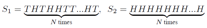
The above observations lead to the conclusion that the small probability of an event may not be an accurate indication that this event is meaningful and we need to take into consideration that the model we use to validate an event describes the randomness of all possible observations. Turning back to the last example of the coin toss, randomness was modeled only by counting the number of H and T in a sequence and not by the probability of a sequence to appear. Taking both issues into account yields the complete model used to describe randomness which is called a contrario model.

Supplementary Material to the related publication

• Example of eliminating circular objects.

  This experimental configuration investigated the efficiency of the method, if it was used to eliminate outliers in a higher semantic level. The problem was to eliminate circular structures (objects) in a collection of objects. The core idea of our method can still be used, since the modeling of a circular object with line segments, would cause the establishment of a large number of short line segments that approximate the circular manifold, compared to the real linear structures, where the corresponding manifolds would provide large line segments. In this experimental analysis, the a-contrario model was differently tuned, compared to the other experiments. The basic parameter that controlled the outcome was the value of b, in the pareto distribution, which is related to the most expected number of points in a line segment. Since we wish to preserve linear structures, this parameter has to have a large value, so as shorter line segments (i.e. those modeling non linear manifolds) can be regarded as non meaningful, and thus, the corresponding points be considered as outliers. The following demonstrates the results of this experiment, by using both the DSaM method [2] and also the widely used polygon approximation (PA) [3]

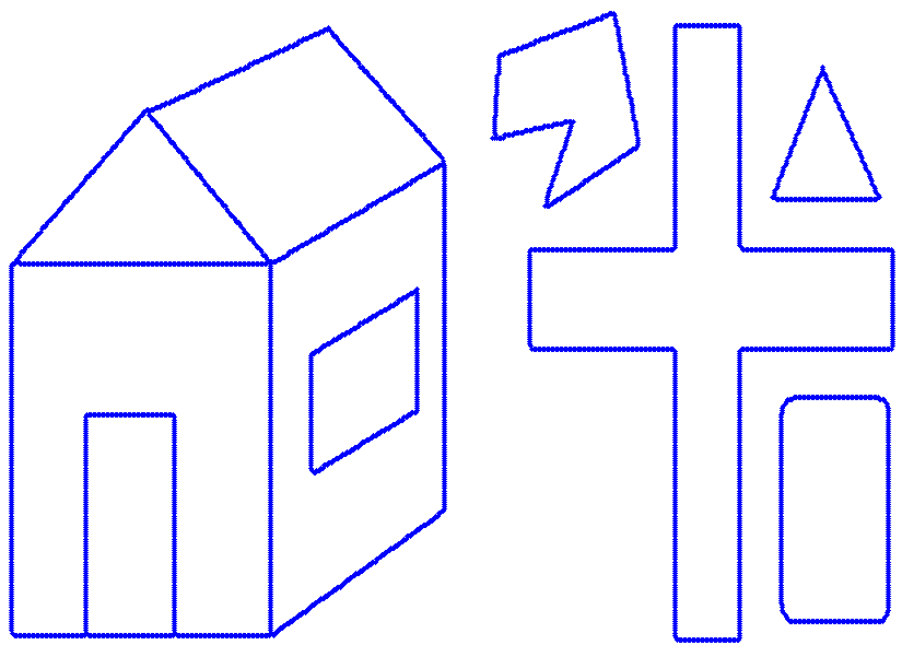
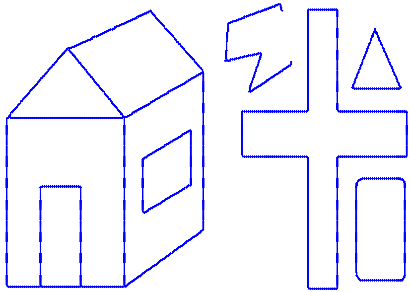
  a	b	c
  Figure 1: An example of eliminating circular structures in a collection of objects. a) The initial image. Result by using b) DSaM, (c) PA.

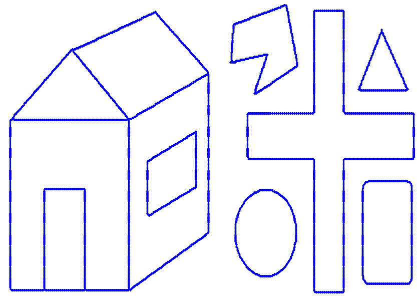
• Example of DSaM modeling of a corrupted set bu outliers and zero mean Gaussian additive noise. The number of outliers is equal to the number of the pure points in the original set

  As it can be seen in the following figure, the DSaM algorithm manages to satisfactorily capture a large number of the initial line segments, while the outliers are modeled with short line segments.

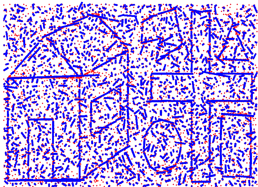
  a	b
  Figure 2: DSaM modeling example. a) General dataset b) Line fitting.

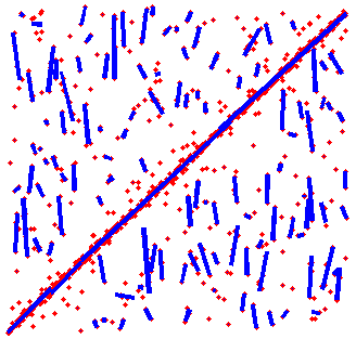
• First and last iterations of the Helmholtz principle framework applied in the line fitting problem.

  The initial data were degraded by zero mean Gaussian additive noise (SNR = 43dB) and outliers were added (the number of outliers is equal to the number of pure points).

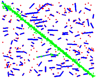
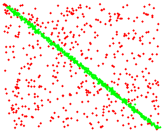
  a	b
  Figure 3: An example of the application of the Helmholtz principle in linear regression. (a) First iteration. The line segments computed are also depicted with blue. (b) Last iteration. Green points depict the points that were considered inliers in each iteration.

• RANSAC configuration details used in the experiments presented in the related paper.

  Considering the RANSAC case the following applies:

  1. The implemented method operates in the polar space, ρ = sin(θ) x + cos(θ) y
  2. The inliers threshold was determined by computing the average distance between neighbors and setting the threshold as a multiple of that distance. The inliers threshold was progressively increased, so as to match the increasing range of outliers. Please note that several configurations of this parameter were examined and the one that kept the best results was employed in our analysis. Moreover, robust statistics was employed for the average computation.
  3. In the related literature, a method for computing an optimal number of iterations is established. Note that, the percentage of outliers is a priori known, as the dataset is artificially degraded. We will explain the worst case (i.e. the number of outliers is equal to the number of pure points). In any other case, the computed results is more accurate. Assume that p is the probability a point is an outlier and n be the minimum number of points needed to establish the model. In our case p=1/2 and n=2 (2 points define a line). Thus, the probability of choosing a sample dataset without outliers is p1=pⁿ=(1/2)²=1/4. Eventually, the optimal number of iterations can be computed as N=log(1-Ps)/log(1-p1), where Ps is the probability of a successful run (i.e. selecting samples without outliers). Based on the desired reliability, Ps can control the final result. In our experiments we fixed N = 1000, which leads to a reliability of the outcome Ps > 0.999999999
  4. The proposed method is the one we used in our implementation of RANSAC.

References

[1] A. Desolneux, L. Moisan, and J. M. Morel. Gestalt theory and computer vision. In Seeing, Thinking and Knowing, volume 38, pages 71–101. Kluwer Academic Publishers, 2004.

[2] D. Gerogiannis, C. Nikou, and A. Likas. Modeling sets of unordered points using highly eccentric ellipses. EURASIP Journal on Advances in Signal Processing, 2014(1):11, 2014.

[3] U. Ramer. An iterative procedure for the polygonal approximation of plane curves. Computer Graphics and Image Processing, pages 244–256, 1972.